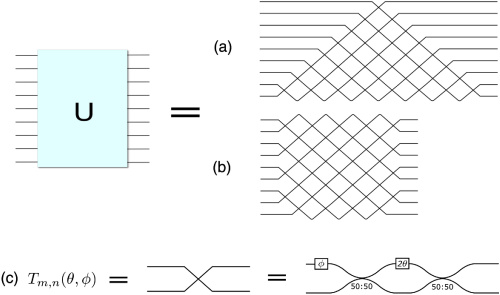
Unitary Matrix Networks in the Time Domain

Imports

# Photontorch
import photontorch as pt

# Python
import torch
import numpy as np
import matplotlib.pyplot as plt
from tqdm.notebook import trange

# numpy settings
np.random.seed(6) # seed for random numbers
np.set_printoptions(precision=2, suppress=True) # show less numbers while printing numpy arrays

Schematic

1. Reck Design

2. Clements Design

Simulation and Design Parameters

Here we will use the matrix network with delays.

N = 4
length = 25e-6 #[m]
transmission = 0.5 #[]
neff = 2.86
env = pt.Environment(
    t_start = 0,
    t_end = 2000e-14,
    dt = 1e-13,
    wl = 1.55e-6,
)
pt.set_environment(env)

source = torch.ones(N, names=["s"])/np.sqrt(N) # Source tensors with less than 4D need to have named dimensions.

env

key	value	description
name	env	name of the environment
t	[0.000e+00, 1.000e-13, ..., 1.980e-11]	[s] full 1D time array.
t0	0.000e+00	[s] starting time of the simulation.
t1	1.990e-11	[s] ending time of the simulation.
num_t	199	number of timesteps in the simulation.
dt	1.000e-13	[s] timestep of the simulation
samplerate	1.000e+13	[1/s] samplerate of the simulation.
bitrate	None	[1/s] bitrate of the signal.
bitlength	None	[s] bitlength of the signal.
wl	1.550e-06	[m] full 1D wavelength array.
wl0	1.550e-06	[m] start of wavelength range.
wl1	None	[m] end of wavelength range.
num_wl	1	number of independent wavelengths in the simulation
dwl	None	[m] wavelength step sizebetween wl0 and wl1.
f	1.934e+14	[1/s] full 1D frequency array.
f0	1.934e+14	[1/s] start of frequency range.
f1	None	[1/s] end of frequency range.
num_f	1	number of independent frequencies in the simulation
df	None	[1/s] frequency step between f0 and f1.
c	2.998e+08	[m/s] speed of light used during simulations.
freqdomain	False	only do frequency domain calculations.
grad	False	track gradients during the simulation

A. Reck Design

nw = pt.ReckNxN(
    N=N,
    wg_factory=lambda: pt.Waveguide(length=1e-4, phase=2*np.pi*np.random.rand(), trainable=True),
    mzi_factory=lambda: pt.Mzi(length=1e-4, phi=2*np.pi*np.random.rand(), theta=2*np.pi*np.random.rand(), trainable=True),
).terminate()

Simulation

detected_time = nw(source)
nw.plot(detected_time[:,0,:,0]); # plot first and only batch

Total power recovered:

detected_time[-1,0,:,0].sum()

tensor(1.0000)

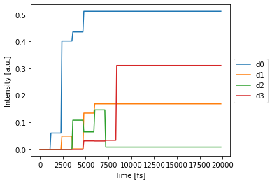
Optimizing the coupling

The goal is to optimize the coupling of the network such that we have the same output at the 4 detectors with an as high as possible amplitude (ideally, higher than in the equal coupling case).

def train_for_same_output(nw, num_epochs=50, learning_rate=0.1):
    target = torch.tensor([1.0/N]*N, device=nw.device)
    lossfunc = torch.nn.MSELoss()
    optimizer = torch.optim.Adam(nw.parameters(), lr=learning_rate)
    with pt.Environment(wl=1.55e-6, t0=0, t1=10e-12, dt=1e-13, grad=True):
        range_ = trange(num_epochs)
        for epoch in range_:
            det_train = nw(source)[-1,0,:,0]
            loss = lossfunc(det_train, target)
            loss.backward()
            optimizer.step()
            range_.set_postfix(loss=loss.item())

train_for_same_output(nw)

Final Simulation

%time det_train = nw(source)
nw.plot(det_train[:,0,:,0]); # plot first and only batch

CPU times: user 42.5 ms, sys: 77 µs, total: 42.6 ms
Wall time: 41.9 ms

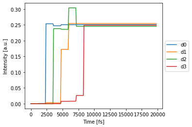
Note that in the Reck network, signals arrive at different times.

Total power recovered

det_train[-1,0,:,0].sum()

tensor(1.)

B. Clements Design

nw = pt.ClementsNxN(
    N=N,
    capacity=N,
    wg_factory=lambda: pt.Waveguide(length=1e-4, phase=2*np.pi*np.random.rand(), trainable=True),
    mzi_factory=lambda: pt.Mzi(length=1e-4, phi=2*np.pi*np.random.rand(), theta=2*np.pi*np.random.rand(), trainable=True),
).terminate()

Simulation

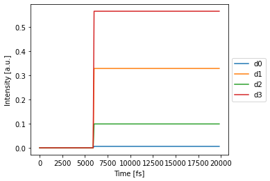
detected_time = nw(source)
nw.plot(detected_time[:,0,:,0]); # plot first and only batch

Total power recovered:

detected_time[-1,0,:,0].sum()

tensor(1.)

Optimizing the coupling

def train_for_same_output(nw, num_epochs=50, learning_rate=0.1):
    target = torch.tensor([1.0/N]*N, device=nw.device)
    lossfunc = torch.nn.MSELoss()
    optimizer = torch.optim.Adam(nw.parameters(), lr=learning_rate)
    with pt.Environment(wl=1.55e-6, t0=0, t1=10e-12, dt=1e-13, grad=True):
        range_ = trange(num_epochs)
        for epoch in range_:
            det_train = nw(source)[-1,0,:,0] # get first and only batch
            loss = lossfunc(det_train, target)
            loss.backward()
            optimizer.step()
            range_.set_postfix(loss=loss.item())

train_for_same_output(nw)

Final Simulation

%time det_train = nw(source)
nw.plot(det_train[:,0,:,0]); # plot first and only batch

CPU times: user 41.1 ms, sys: 21 µs, total: 41.1 ms
Wall time: 40.4 ms

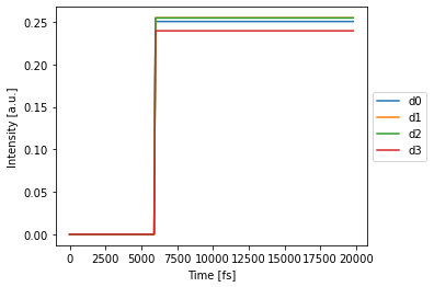
Note that in the Clements network, all signals arrive at the same time at the detector.