Circuit optimization by backpropagation with PyTorch
Imports
[1]:
# Python
%matplotlib inline
import numpy as np
import matplotlib.pyplot as plt

# Torch
import torch

# PhotonTorch
import photontorch as pt

# Progress Bars
from tqdm.notebook import tqdm
Michelson Interferometer Cavity
Simulation and Design Parameters
[2]:
neff = np.sqrt(12.1)
wl = 1.55e-6
dt = 0.5e-9
total_time = 2e-6
time = np.arange(0,total_time,dt)
Network
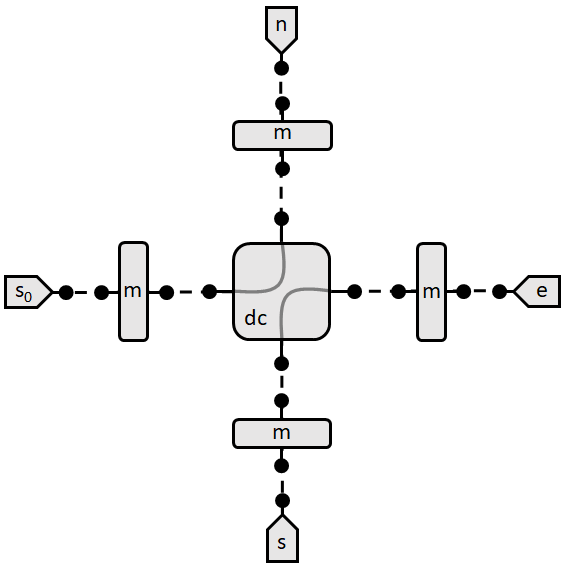
We define the network again in the standard way. However, sometimes it is useful to define components only once, but save copies of the component while setting it as an attribute of the network.
Look for example at the line
self.m_west = self.m_north = self.m_east = self.m_south = pt.Mirror(R=0.9)
Note that the order of the detectors is defined by where they appear in the link.
[3]:
# define network in the standard way:
class MichelsonCavity(pt.Network):
    def __init__(self):
        super(MichelsonCavity, self).__init__()
        self.west = pt.Source()
        self.north = self.east = self.south = pt.Detector()
        self.m_west = pt.Mirror(R=0.9)
        self.m_north = pt.Mirror(R=0.9)
        self.m_east = pt.Mirror(R=0.9)
        self.m_south = pt.Mirror(R=0.9)
        self.wg_west = pt.Waveguide(0.43, neff=neff, trainable=False)
        self.wg_north = pt.Waveguide(0.60, neff=neff, trainable=False)
        self.wg_east = pt.Waveguide(0.95, neff=neff, trainable=False)
        self.wg_south = pt.Waveguide(1.12, neff=neff, trainable=False)
        self.dc = pt.DirectionalCoupler(coupling=0.5, trainable=False)
        self.link('west:0','0:m_west:1', '0:wg_west:1', '0:dc:2', '0:wg_east:1', '0:m_east:1', '0:east')
        self.link('north:0', '0:m_north:1', '0:wg_north:1', '1:dc:3', '0:wg_south:1', '0:m_south:1', '0:south')

# create network
nw = MichelsonCavity()

# print out the parameters of the network:
for p in nw.parameters():
    print(p)
BoundedParameter in [0.00, 1.00] representing:
tensor(0.9000)
BoundedParameter in [0.00, 1.00] representing:
tensor(0.9000)
BoundedParameter in [0.00, 1.00] representing:
tensor(0.9000)
BoundedParameter in [0.00, 1.00] representing:
tensor(0.9000)
Simulation
[4]:
%%time
with pt.Environment(wl=wl, t=time):
    detected = nw(source=1)[:,0,:,0] # get all timesteps, the only wavelength, all detectors, the only batch
CPU times: user 1.1 s, sys: 59.7 ms, total: 1.16 s
Wall time: 581 ms
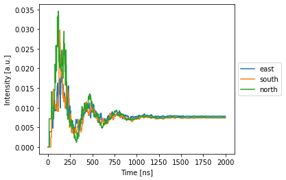
[5]:
nw.plot(detected);
Training
Training parameters:
[6]:
num_epochs = 10 # number of training cycles
learning_rate = 0.2 # multiplication factor for the gradients during optimization.
lossfunc = torch.nn.MSELoss()
optimizer = torch.optim.Adam(nw.parameters(), learning_rate)
We would like to train the network to arrive in another steady state with the same output everywhere:
[7]:
total_power_out = detected.data.cpu().numpy()[-1].sum()
target = np.ones(3)*total_power_out/3
# The target should be a torch variable.
# You can create a new torch variable with the right type and cuda type, straight from the network itself:
target = torch.tensor(target, device=nw.device, dtype=torch.get_default_dtype())
Now we can start the training. However, to be able to train the parameters of the network, gradient tracking should be enabled in the simulation environment. This is done by setting the enable_grad flag to True.
[8]:
# loop over the training cycles:
with pt.Environment(wl=wl, t=time, grad=True):
    for epoch in tqdm(range(num_epochs)):
        optimizer.zero_grad()
        detected = nw(source=1)[-1,0,:,0] # get the last timestep, the only wavelength, all detectors, the only batch
        loss = lossfunc(detected, target) # calculate the loss (error) between detected and target
        loss.backward() # calculate the resulting gradients for all the parameters of the network
        optimizer.step() # update the networks parameters with the gradients
        del detected, loss # free up memory (important for GPU)
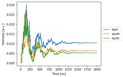
Do a final simulation:
[9]:
with pt.Environment(wl=wl, t=time):
    detected = nw(source=1) # get all timesteps, the only wavelength, all detectors, the only batch
    nw.plot(detected);