Simulating an All-Pass Filter

Imports

%matplotlib inline
import numpy as np
import matplotlib.pyplot as plt
import photontorch as pt

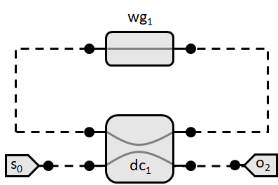
Schematic

Simulation & Design Parameters

dt = 1e-14 # Timestep of the simulation
total_time = 2.5e-12 # Total time to simulate
time = np.arange(0, total_time, dt) # Total time array
loss = 1 # [dB] (alpha) roundtrip loss in ring
neff = 2.34 # Effective index of the waveguides
ng = 3.4
ring_length = 1e-5 #[m] Length of the ring
transmission = 0.5 #[] transmission of directional coupler
wavelengths = 1e-6*np.linspace(1.5,1.6,1000) #[m] Wavelengths to sweep over

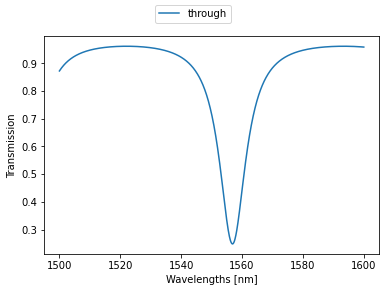
Frequency Domain Analytically

As a comparison, we first calculate the frequency domain response for the all-pass filter analytically: \begin{align*} o = \frac{t-10^{-\alpha/20}\exp(2\pi j n_{\rm eff}(\lambda) L / \lambda)}{1-t10^{-\alpha/20}\exp(2\pi j n_{\rm eff}(\lambda) L / \lambda)}s \end{align*}

def frequency():
    ''' Analytic Frequency Domain Response '''
    detected = np.zeros_like(wavelengths)
    for i, wl in enumerate(wavelengths):
        wl0 = 1.55e-6
        neff_wl = neff + (wl0-wl)*(ng-neff)/wl0 # we expect a linear behavior with respect to wavelength
        out = np.sqrt(transmission) - 10**(-loss/20.)*np.exp(2j*np.pi*neff_wl*ring_length/wl)
        out /= (1 - np.sqrt(transmission)*10**(-loss/20.)*np.exp(2j*np.pi*neff_wl*ring_length/wl))
        detected[i] = abs(out)**2
    return detected

def plot_frequency(detected, **kwargs):
    ''' Plot detected power vs time '''
    labels = kwargs.pop('labels', ['through','drop','add'])
    plots = plt.plot(wavelengths*1e9, detected, **kwargs)
    plt.xlabel('Wavelengths [nm]')
    plt.ylabel('Transmission')
    if labels is not None: plt.figlegend(plots, labels, loc='upper center', ncol=len(labels)%5)
    plt.show()

%time detected_target = frequency()
plot_frequency(detected_target)

CPU times: user 8.9 ms, sys: 0 ns, total: 8.9 ms
Wall time: 8.9 ms

Photontorch

Next, we try to do the same simulation with Photontorch:

A Photontorch network - or circuit - is created by subclassing the Network class. First all network subcomponents are defined as attributes of the network, after which the ports of the subcomponents can be linked together by using the link method.

The link method takes an arbitrary number of string arguments. Each argument contains the component name together with a port number in front of and a port number behind the name (e.g. "0:wg:1"). The port number behind the name will connect to the port number in front of the next name. The first component does not need a port number in front of it, while the last component does not need a port number behind.

The port order of each of the standard Photontorch components can be found in its docstring. Try for example this in a code cell:

?DirectionalCoupler

Define Allpass Network

class AllPass(pt.Network):
    def __init__(self):
        super(AllPass, self).__init__() # always initialize first.
        self.src = pt.Source()
        self.wg_in = pt.Waveguide(0.5*ring_length, neff=neff, ng=ng)
        self.dc = pt.DirectionalCoupler(1-transmission)
        self.wg_through = pt.Waveguide(0.5*ring_length, neff=neff, ng=ng)
        self.wg_ring = pt.Waveguide(ring_length, loss=loss/ring_length, neff=neff)
        self.det = pt.Detector()
        self.link('src:0', '0:wg_in:1', '0:dc:1', '0:wg_through:1', '0:det')
        self.link('dc:2', '0:wg_ring:1', '3:dc')

Create AllPass Network

nw = AllPass()

Time Domain Simulation

Setting the simulation environment

A simulation cannot be performed before a simulation environment is set. The simulation environment contains all the necessary global information (such as wavelength, timestep, number of timesteps, …) to perform a simulation.

After the environment is set, a simulation can be run (for example for a source with constant amplitude)

# create environment
environment = pt.Environment(
    wl=np.mean(wavelengths),
    t=time,
)

# set environment
pt.set_environment(environment)

# run simulation
detected = nw(source=1)

Notice the shape of the detected tensor:

detected.shape

torch.Size([250, 1, 1, 1])

In general the shape of the detected tensor always has the same form:

(# timesteps, # wavelengths, # detectors, # parallel simulations)

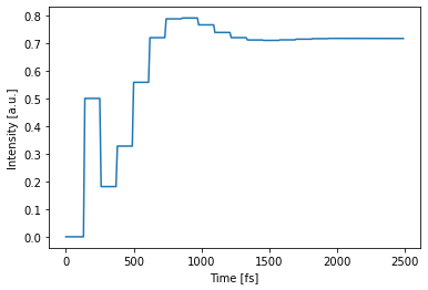
In this case, we did a single simulation for 2500 timesteps while only using a single wavelength and a single detector.

Each network has a plotting function, which uses this information and the information in the current environment to give you the most helpful plot possible. In this case, it is a simple power vs time plot:

# plot result
nw.plot(detected);

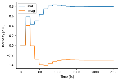
Sometimes, it is useful to detect the complex field values in stead of the power. This can be done by setting the power=False flag during simulation:

detected = nw(source=1, power=False)
print(detected.shape)

torch.Size([2, 250, 1, 1, 1])

In this case, an extra dimension of size 2 will be added in front of the original detected shape, giving the real and imaginary part of the deteced field (because PyTorch does not support imaginary tensors).

nw.plot(detected[0])
nw.plot(detected[1])
plt.legend(['real', 'imag'])
plt.show()

Frequency Domain Simulation

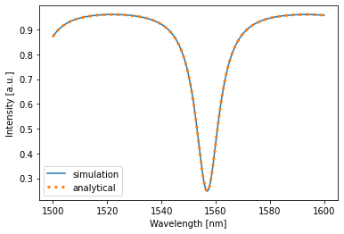
Setting up a frequency domain simulation is very similar to setting up a time domain simulation. The only difference actually happens in the simulation environment, where the frequency_domain flag was set to True. This will remove all the delays inside the simulation, after which a simulation is performed for a single timestep. Because all the internal delays of the network were set to zero, this simulation of a single timestep will immediately reach the steady state. This is a very fast method for calculating the frequency domain response of your circuit.

In the following, we choose to set the environment with a context manager. This will ensure the environment is closed after exiting the with-block. This way, the environment will return to the environment which was set originally.

# create simulation environment
with pt.Environment(wl=wavelengths, freqdomain=True) as env:
    detected = nw(source=1)
    print("This was detected inside the context manager:\n"
          "We see an exact copy of the analytically predicted response, as is to be expected")
    nw.plot(detected, label="simulation")
    plt.plot(env.wavelength*1e9, detected_target, linestyle="dotted", linewidth=3, label="analytical")
    plt.legend()
    plt.show()

print("This was detected outside the context manager, "
      "with the default environment:")
detected = nw(source=1)
nw.plot(detected)
plt.show()

This was detected inside the context manager:
We see an exact copy of the analytically predicted response, as is to be expected

This was detected outside the context manager, with the default environment:

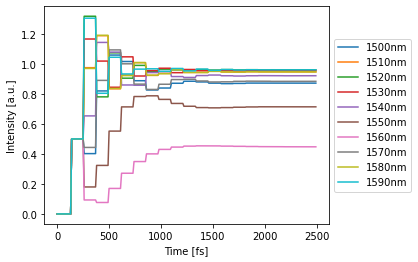
Multimode Simulation

One of the strengths of photontorch, is that time-domain simulations can be done for multiple wavelengths at the same time. Just specify a range of wavelengths to simulate over in the simulation environment

with pt.Environment(wl=wavelengths[::100], t=time):
    detected = nw(source=1)
    nw.plot(detected);