Simulating an Add-Drop Filter

Imports

%matplotlib inline
import numpy as np
import matplotlib.pyplot as plt
import photontorch as pt

Simple Add Drop filter

Simulation & Design Parameters

dt = 1e-14 #[s]
total_time = 2000*dt #[s]
time = np.arange(0, total_time, dt)
c = 299792458 #[m/s]
ring_length = 50e-6 #[m]
transmission = 0.7 #[]
wavelengths = 1e-6*np.linspace(1.50, 1.6, 1000) #[m]

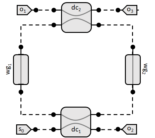
Circuit

In the all-pass notebook, we saw how to create a network by subclassing pt.Network. Although this is the preferred way of creating a network, sometimes you want to get rid of the boilerplate of creating a network. This can be done by creating the network using a context manager:

with pt.Network() as nw:
    nw.term_in = pt.Source()
    nw.term_pass = nw.term_add = nw.term_drop = pt.Detector()
    nw.dc1 = nw.dc2 = pt.DirectionalCoupler(1-transmission)
    nw.wg1 = nw.wg2 = pt.Waveguide(0.5*ring_length, loss=0, neff=2.86)
    nw.link('term_in:0', '0:dc1:2', '0:wg1:1', '1:dc2:3', '0:term_drop')
    nw.link('term_pass:0', '1:dc1:3', '0:wg2:1', '0:dc2:2', '0:term_add')

Simulate Time Domain

with pt.Environment(wl=np.mean(wavelengths), t=time):
    detected = nw(source=1)
    nw.plot(detected);

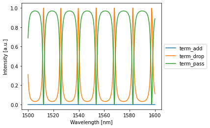
Simulate Frequency Domain

with pt.Environment(wl=wavelengths, freqdomain=True):
    detected = nw(source=1)
    nw.plot(detected)

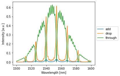
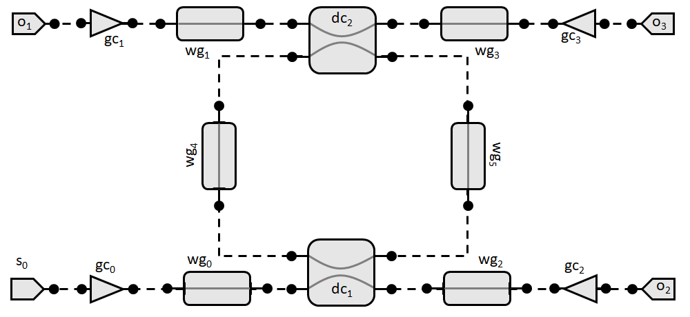
Add Drop Filter With Grating Couplers

Simulation & Design Parameters

dt = 1e-14 #[s]
total_time = 1000*dt #[s]
time = np.arange(0, total_time, dt)

distance_x = 100.0e-6 #[m]
distance_y = 30.0e-6 #[m]
center_wavelength=1.55e-6 #[m]
bandwidth=0.06e-6 #[m]
peak_transmission=0.60**0.5
reflection=0.05**0.5

c = 299792458 #[m/s]
wg_length = 89.22950569e-6 #[m]
ring_length = 50e-6 #[m]
transmission = 0.7 #[]
wavelengths = 1e-6*np.linspace(1.50, 1.6, 1000) #[m]

Circuit

with pt.Network() as nw:
    # components
    nw.src = pt.Source()
    nw.through = nw.add = nw.drop = pt.Detector()
    nw.dc1 = nw.dc2 = pt.DirectionalCoupler(1 - transmission)
    nw.wg1 = nw.wg2 = pt.Waveguide(0.5 * ring_length, loss=0, neff=2.86)
    nw.wg_in = nw.wg_through = nw.wg_add = nw.wg_drop = pt.Waveguide(
        length=wg_length, loss=0.0, neff=2.86, trainable=True
    )
    nw.gc_in = nw.gc_through = nw.gc_add = nw.gc_drop = pt.GratingCoupler(
            R=reflection,
            R_in=0,
            Tmax=peak_transmission,
            bandwidth=bandwidth,
            wl0=center_wavelength,
        )

    # links
    nw.link('src:0', '0:gc_in:1', '0:wg_in:1', '0:dc1:2', '0:wg2:1',
            '1:dc2:3', '1:wg_drop:0', '1:gc_drop:0', '0:drop')

    nw.link('through:0', '0:gc_through:1', '0:wg_through:1', '1:dc1:3', '0:wg1:1',
            '0:dc2:2', '1:wg_add:0', '1:gc_add:0', '0:add')

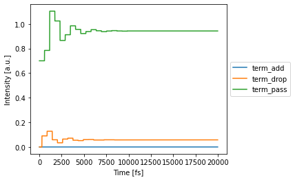
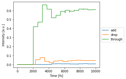
Simulate Time Domain

with pt.Environment(wl=np.mean(wavelengths), t=time):
    detected = nw(source=1)
    nw.plot(detected);

Simulate Frequency Domain

with pt.Environment(wl=wavelengths, freqdomain=True):
    detected = nw(source=1)
    nw.plot(detected)